It works similarly to a breadth first search style algorithm where it branches out from a starting point and checks nodes closest to the start first.
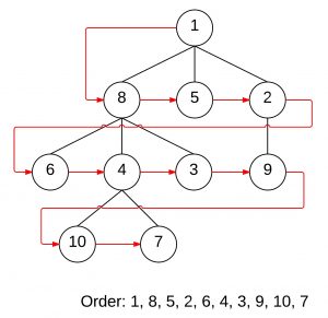
Like in the illustration, it starts by checking the immediate neighbors first (8, 5, and 2, since they are directly connected). In the next iteration it checks all of the immediate neighbors of the nodes it just checked, and repeats these iterations until it finds a result.
However, it needs to remember which nodes it needs to check next. That is where the open list comes in. When it checks a node it will take all of that node’s neighbors and throw them in the open list so that they can be checked later. There are two potential problems with this though:
- This naive approach might lead it to checking the same node multiple times
- If the insertion into the open list isn’t done carefully, then it might insert nodes for checking in the wrong order, changing it from a breadth first search into a depth first search, or (effectively) random order search.
In order to solve problem 1, a closed list is added to check for duplicate node checks. This will prevent it from backtracking to the start through a well searched area and prevent it from exponentially exploding, searching and re-searching the same nodes over and over.
To solve problem 2, a priority queue is used for the open list to sort nodes by importance. This prevents the open list from becoming jumbled by insertions and keeps the algorithm on the right path. The algorithm should search closer nodes first, so the queue sorts should sort by distance and put smaller nodes up front. The implementation of the queue itself doesn’t matter as much, as long as it works, so it can be anything from a sorted array, to a heap, or even a bucket based container for fast interactions.
The last bit about priority is an important part of A* since it is what separates A* from its “parent” algorithm Dijkstra. The priority, the distance, introduces a numerical score that can be manipulated to make it run faster. The difference between Dijkstra and A* is that A* changes the priority queue’s score a little by adding in a heuristic, an estimation to guess at where it should search next instead of blindly branching out. Without a heuristic Dijkstra looks like an even outwards spread like so:
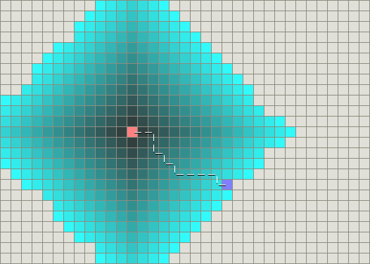
While A* can use distance to the goal in a heuristic to weigh the scores towards moving to the goal:
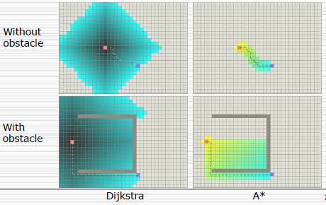
A* can do this with its extra heuristic by calculating the distance to the goal, and adding the distance to the overall score of a node turning the node score equation from score = distanceFromStart (Dijkstra) to score = distanceFromStart + distanceFromEnd (A*, distanceFromEnd is the heuristic).
It isn’t a perfect solution, so in some situations A* may actually end up being slower than Dijkstra, but in the majority of cases it can speed of the search tremendously. The search can also be made faster by making the heuristic estimate “too far”, sacrificing the accuracy and guarantee of an exact shortest path for a faster to find path.
A* also has the added benefit of adding things like environmental weights, increasing the cost to move through certain areas like tar pits, or reducing weight of areas like healing zones. What you do with it exactly is up to you.
As a side note, it looks like neighbor.h is your code’s heuristic, neighbor.g is your code’s cost, and neighbor.f is the final score for the open list.
Edit: Forgot to mention that visited nodes are marked with the node that was used to travel to them so that the path itself can be traced back starting from the end. The path is built by taking the end node and reconstructing it using references to previously visited nodes.
Also the use of a heuristic messes with the numbers a little, so a node that was previously searched may be reached again from a more optimal location, so A* adds a little rule that allows nodes on the closed list to be revisited if a better path is found. This may introduce some backtracking, but the reduced cost of node searches should offset that extra cost.


