If you’re looking to make a cruise control similar to how real vehicles function, you’ll want to research something called a PID loop. They’re used a lot in the real world when automatic control of physical things is required (cruise control, air conditioning, robotics, etc.).
This graphic is a good representation of PID control, but it’s a little confusing if you don’t know anything about PID, so I’ll try to explain. The basic premise of PID control is that you have some wheel, or valve, or mechanical thing which needs to do something precisely (spin at a certain speed, maneuver to a certain position, etc.). Normally it’s very hard to control that thing reliably. PID theory is the solution to reliable control.
PID Visualized

Imagine you have a motor connected to a fan which cools you off on a hot summer day. Currently, your motor is not spinning, but you want to get the motor spinning so that it will cool you off. To get the motor spinning, you apply an electrical charge to the motor: the more charge you apply the faster it will spin. Your problem, though, is that it’s not easy to control the fan manually. If the fan spins too fast, your hat (which is keeping the sun off your head) will blow away. If the fan spins too slow, you won’t cool off. This is where PID theory comes in.
PID is something known as a control loop, which means that it makes very small adjustments to a measured value (speed, position, etc.) over short intervals (loops) to get achieve a desired value. In this case, you’re trying to get your motor to spin at just the right speed.
The image is a representation of a PID loop. On the left is the term r(t) which stands for the desired value, in this case the perfect fan speed. On the right hand side is the term y(t) which stands for the measured value AKA the current speed of the fan.
A PID loop begins at the first yellow circle on the left. The measured value is subtracted from the desired value to find e(t): the error. After the error is found, three individual operations are performed based on it. In the green rectangle is the proportional operation. The proportional operation multiplies the error by the proportional constant, which is just a number less than 1. I’m going to call the result of the operation P.
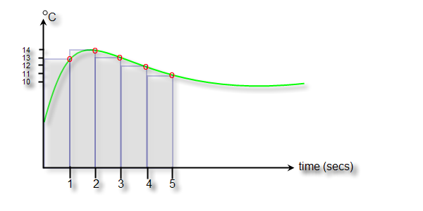
In the blue rectangle is the integral operation and is probably the most convoluted (and the operation the video you linked was referring to). Integral is a fancy calculus term for the area between a curve and the x-axis of a graph. In the blue rectangle, the integral is calculated by (1.) Graphing all of the separate errors in the y-axis (remember that we’re “looping” very quickly, so we keep track of each error from the previous loop), and using the x-axis to represent the amount of time which has passed. (2.) Finding the area under the curve formed by the graph. This image is a good way to visualize what I just said. The integral(area under the curve) is then multiplied by a decimal called the integral constant to get a final number that I’ll call I.
The final rectangle, the orange one, represents an operation called the derivative. The derivative is another fancy calculus term which refers to the slope of a curve. Although there are a lot of complicated ways to explain how to find the derivative, but in a simple PID loop the only things that matter are the current error, and the error from the last loop of the PID controller. To find the derivative, you divide the change in error (current - last) by the amount of time between loops. The derivative is then multiplied by a decimal called the derivative constant and creates a number I’ll call D.
The final mathy operation of a PID loop is the easiest to comprehend: you simply add the 3 rectangles together. P + I + D = the power you supply to the fan! The beauty of a PID loop is that because it constantly adjusts the power to the fan, it’s self-regulating.
Hopefully, this is a good introduction to PID theory.
(now I’m going to bed  )
)

