More Complex Neural Networks

inpad_2 · August 21, 2022, 3:28pm

Introduction

I have already written two tutorials about neural networks

Understanding Neural Network Backpropagation Learning Algorithm - Resources / Community Tutorials - DevForum | Roblox

An introduction to Perceptrons - Bulletin Board - DevForum | Roblox

but both of them explain the math and the concepts of forward propagation and backward propagation based on a perceptron(which is a simplified neural network). This is why, I thought that writing a tutorial about neural networks that are more complex and consist of more neurons and layers is essential.

Prerequisites

A basic idea of what a neural network is (This tutorial is not an introduction to neural networks!)
Basic calculus knowledge will help a lot (you should at least know what a derivative is, else see the following )

What is the derivative of a function

What is the derivative?

Consider a function y = f(x).

We call the increase Δx of a variable x its change, as x increases or decreases from a value x = x0 to an other value x = x1. Therefore Δx = x1- x0, which can be written as x1 = x0 + Δx (Note: y1 = f(x1) = f(x0 + Δx)). If the variable x is changing by Δx from a value of x=x0( that is if x changes from x=x0 to x = x0 + Δx) then the function will change by Δy = f(x0 + Δx) - f(x0) from the value y = f(x0) (that is the same with saying y1 - y0=Δy or f(x1) - f(x0) = Δy ). The quotient Δy / Δx = Change in y/ Change in x is called the instantaneous rate of change of the function

The derivative of a function y=f(x) with respect to x is defined by the following:

The essence of calculus is the derivative . The derivative is the instantaneous rate of change of a function with respect to one of its variables. This is equivalent to finding the slope of the tangent line to the function at a point.

Because it is really time consuming to use the formula above every time we need to find the derivative of a function, there are luckily for us some formulas which we can use. An example of these is given in the following image:

Note that f’(x) and dy/dx(when we have an equation y=f(x)) symbolizes the derivative of a function f(x).

There are also some rules that we need to take into consideration when trying to find the derivative of a function.

For example if we want to find the derivative of a function y=f(u) and u = g(x) with respect to x then the derivative of the function y=f(u) with respect to x is the following:

This is known as the chain rule.

Other rules are the following:

Notation

m = size of the training set
n = amount of input variables
l = specific layer
w = weights
b = bias
single input variable

What are partial derivatives

The reason why there is a new type of derivative (partial derivatives) is that when the input of a function is made up of multiple variables like f(x,y) = x^2 + cos(y) we want to see how the function changes as we just let just one of those variables change while we hold the others constant.

For example the derivative of the function we saw earlier f(x) = x^2 + cos(y) has two partial derivatives. One with respect to x, and one with respect to y.

The derivative of the function f(x,y) with respect to x is the following:

while the derivative of the same function with respect to y is the following:

As you have probably guessed , to find the partial derivative of a function that its input is made up of multiple variables with respect to one variable you just treat all the other variables as constants and find the derivative. In the above function, when finding the derivative with respect to x, we treat cos(y) as a constant and this is why it becomes 0 (the derivative of a constant is 0).

If you see this for the first time, see this article to understand the concept of partial derivatives better Introduction to partial derivatives (article) | Khan Academy or this Partial derivative - Wikipedia .

Neural network Architecture

Let’s consider the above neural network. it consists of two layers, two inputs and the hidden layer has three neurons. Each neuron has assigned the weight parameter (w11, w12, w13, w21, w22, w23, w31, w41, w51) . The bias b1 and b2 as you can see are the bias parameter of the input layer and the hidden layer. You will probably wonder what is this number that each weight has. While you might think that for example the weight w11 has the number eleven that is not the case.

Actually it has two numbers, that represent different things(1,1). The first one represents we are looking at the weight that “comes” from the first node while the second one represents that the weight is “going” to the first node of the second layer. let’s see another example: the weight w41. Again two different numbers (4,1). the first one shows that we are looking to the weight that “comes” from the 4th node while the second one represents that the weight is “going” to the first node of layer 3.

What steps does a Neural network follow?

Weights and bias parameters initialization
Forward Propagation
Loss Computing
Back-propagation
Weights and bias parameters updating

Forward propagation

In forward propagation, the input data are fed to the network in the forward direction hence the name forward-propagation.

Firstly, all the weights and the inputs that are connected to each neuron in the first layer are multiplied and then summed and then the bias is added. In our case

z11 = (x1w11) + (x2w21) + b1
z12 = (x1w12) + (x2w22) + b1
z13 = (x1w13) + (x2w23) + b1

We usually name the result z, but you can name it however you want. it is good though to follow a specific notation so there are no misunderstandings.

Then, we pass the results in an activation function (let’s say sigmoid). The activation function that you will use in the neural network is up to you. Some choices are the following:

anyway, the results in our example are the following:

|a11 = σ (z11)|
|a12 = σ (z12)|
|a13 = σ (z13)|
where σ(x) is the activation function. In this tutorial we will use the sigmoid activation function.

Now, there is one additional layer, the output layer so we repeat the process with a small difference. Our inputs are the results we found above (a11, a12, a13). So what we do, is we sum the products of weights and the inputs that are connected to our neuron and add the bias b2.

z21 = a11w31 + a12w41 +a13*w51+ b2

Then like before we pass the result to our activation function, so our result is:

a21 = σ (z21)

and we have finally finished our two first steps. You might ask 'hey but we did not initialize any weights or biases" but I will answer that they are completely random and so it is up to you to initialize them.

Loss computing

We use the following function:

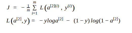
The main goal of the neural network is to get the minimum error(loss). We can achieve a minimum error between an actual target value and predicted the target value if we get the correct value of the weight and bias parameters.

Backpropagation

So, the error is changed with respect to the parameters. This rate of change in error is to be found by calculating partial derivation of the loss function with respect to each parameter. By performing derivation, we can determine how sensitive is the loss function to each weight and bias parameters. This method is also known as Gradient Descent optimization method.

So let’s see what we actually did in the forward propagation and what we will do in the backpropagation :

z[layer1] = w[layer1] * input[layer1] + bias1 => a[layer1] = σ(z[layer1]) => z[layer2] = w[layer2] * a[layer1] + b2 => a[layer2] = σ(z[layer2]) => L(a[layer2],y)

this is what we did in forward propagation and error computing. Notice that it is a general form and for example z[layer1] means [z11,z12,z13] so it would be wrong to assume that it is one value. What backpropagation does is the opposite of forward propagation:

L(a[layer2],y) => da[layer2] => dz[layer2] => da[layer1] => dz[layer1]

The da[layer2], dz[layer2], dw[layer2], db[layer2], da[layer2], dz[layer1], dw[layer1] and db[layer1] are the partial derivation of the loss function with respect to a[layer2], z[layer2], w[layer2], b[layer2], a[layer1], z[layer1], w[layer1] and b[layer1] respectively

I remind you that for example z[layer2] is not one value but all the z values in the layer2

Let’s see the calculation partial derivation of weight and bias parameters with respect to those parameters.

With respect to da[layer2] ( we will from now on symbolize it as da^[2])

With respect to dz^[2]

I have assumed that we have used the sigmoid activation function

With respect to dw^[2]
With respect to db^[2]
With respect to da^[1]
With respect to dz^[1]

Where σ’() is the derivative of the sigmoid function
With respect to w^[1]

with respect to db^[1]

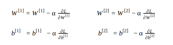
Weight and bias updating

The weight and bias parameters are updated by subtracting the partial derivation of the loss function with respect to those parameters.

Here α is the learning rate that represents the step size. It controls how much to update the parameter. The value of α is between 0 to 1.

Sources

Future Changes

nothing yet

Recommended resources

If you want to learn more about neural Networks and have an even more mathematical approach check this video The Complete Mathematics of Neural Networks and Deep Learning - YouTube